R
Script for Calculating the Brainerd-Robinson Coefficient of Similarity and Assessing
Sampling Error
This document can be cited
as follows:
Society for American Archaeology style:
Peeples, Matthew A.
2011 R Script for Calculating the Brainerd-Robinson Coefficient of Similarity
and Assessing Sampling Error. Electronic document, http://www.mattpeeples.net/br.html,
accessed
APA style:
Peeples, Matthew A. (2011) R Script for Calculating the Brainerd-Robinson Coefficient
of Similarity and Assessing Sampling Error. [online]. Available: http://www.mattpeeples.net/br.html.
(
)
Brainerd Robinson Coefficient of Similarity:
The Brainerd-Robinson (BR) coefficient is a similarity measure that was developed
within archaeology specifically for comparing assemblages in terms of the proportions
of types or other categorical data. Although this measure is commonly used in
archaeological studies, it cannot be calculated with most commercial software
packages. This script calculates BR coefficients on count or percent data. Further,
following procedures first described by DeBoer, Kintigh, and Rostoker (1996),
this script also calculates the probabilities of obtaining a BR similarity value
less than or equal the actual value by chance for every pair-wise comparison.
These probability values can be useful in determing when differences between
sites might be a function of sampling error and when they are likely not. This
probability assessment is described in more detail below.
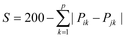
BR is a city-block metric of similarity (S) that is calculated as:
where, for all variables (k), P is the total percentage in assemblages i and
j. This provides a scale of similarity from 0-200 where 200 is perfect similarity
and 0 is no similarity.
This remainder of this document provides a brief overview of the BR.R script.
This script is based on the BRSAMPLE originally written by Keith Kintigh as
part of the Tools for Quantitative
Archaeology program suite. You can download a sample data
file along with the script to follow along
with this example. Right click and click Save As for both of the files above.
The sample data used here are based on Huntley's (2004, 2008) ceramic compositional
study focused on the Zuni region. The discussion and interpretations of the
sample data presented below are also based on Huntley's published work.
File Format:
This script is designed to use the *.csv (comma separated value) file format.
Microsoft Excel as well as the open-source program Calc in the Open
Office suite can be used to produce files in this format from any tabular
data. For the purposes of this script, the file should be named "BR.csv".
Note that file names are case sensitive. The text of the script file may be
edited to change the input file name.
Table Format:
Tables should be formatted with each of the samples/sites/observations as rows
and each of the categorical variables as columns. The first row of the spreadsheet
should be a header that labels each of the columns. The first column should
contain the name of each unit (i.e., level, unit, site, etc.). Row names may
not be repeated. All of the remaining columns should contain numerical count
or percent data. The sample data from Huntley's (2004, 2008) study consist of
counts of 5 ceramic compositional groups from 9 sites in the Zuni region :
SITE
DLH-1
DLH-2a
DLH-2b
DLH-2c
DLH-4
Atsinna
16
9
3
0
1
Cienega
13
3
2
0
0
Mirabal
9
5
2
5
0
PdMuertos
14
12
3
0
0
Hesh
0
26
4
0
0
LowPesc
1
26
4
0
0
BoxS
0
11
3
13
0
OjoBon
0
0
17
0
16
Sp170
0
0
18
0
14
Requirements
for Running the Script: In order to run this
script, you must install the R statistical package (version 2.8 or later). R
can be downloaded for free here. Follow
the instructions on the R site for installation procedures. In addition to this,
this script requires one specific R packages to be installed (statnet). In order
to install this package, simply click on the "packages" drop down
menu at the top of the R window and click on "Install package(s)".
Choose a CRAN mirror (it is best to choose the location closest to you). Select
the "statnet" package and click OK. For further instructions for installing
packages, check here.
Starting the Script: The first step for running the script is to place the script file "BR.R"
and the data file "BR.csv" in the working directory of R. To change
the working directory, click on "File" in the R window and select
"Change dir", then simply browse to the directory that you would like
to use as the working directory. Next, to actually run the script, type the
following line into the R command line:
source('BR.R')
Running the Script: After typing the command
above into the command line, the console will request user input with two prompts.
1) Are the
data percents or counts? 1=percents, 2=counts:
At this prompt enter 1 if input data
are percents. For percent data, the script will output a rectangular matrix
of BR values for all pair-wise comparisons and then end without running the
sampling error assessment (which requires count data). If the data are counts,
a second prompt will appear.
2) How many
random runs :
At this prompt, enter the number of
random runs that you wish use to assess sampling error. Increasing the number
of random runs increases the total time it will take to calculate probabilities.
Most relatively recent computers (should be able to calculate 1,000 runs in
a few seconds to several minutes depending on the size of the original data
table.
Output: After the script has run, one or two files will be placed in the R
working directory depending on whether percent or count data were input.
For both percent and count data, a file named "BR_out.csv" will be
output. This file is a rectangular matrix of Brainerd-Robinson similarity coefficients
for all sites/samples included. The sample output is shown below. Numbers shown
in red in the table below represent comparisons between sites in the
same settlement cluster and comparisons in black represent comparisons between
settlement clusters. Data will not be color coded in the actual output.
Atsinna
Cienega
Mirabal
PdMuertos
Hesh
LowPesc
BoxS
Ojo Bon
S170
Atsinna
200
164
152
179
83
89
83
28
28
Cienega
164
200
138
151
56
62
56
22
22
Mirabal
152
138
200
152
67
73
114
19
19
PdMuertos
179
151
152
200
103
110
102
21
21
Hesh
83
56
67
103
200
194
104
27
27
LowPesc
89
62
73
110
194
200
104
26
26
BoxS
83
56
114
102
104
104
200
22
22
Ojo Bon
28
22
19
21
27
26
22
200
191
S170
28
22
19
21
27
26
22
191
200
If the input data are counts, a
second file named "BR_prob" will also be created. This file is a rectangular
matrix of probability values based on the Monte Carlo simulation procedure described
below. In this table, a value of 0 indicates a probability less than the number
of significant digits considered. For example, if probabilities were calculated
to thousandths (i.e., 0.115), a value of 0 indicates some value < 0.001.
The sample output table should be similar to the table shown below. Actual values
will vary somewhat do to the randomization procedure. The sample output shown
here was calculated based on 1,000 random runs. Again, numbers shown
in red in the table below represent comparisons between sites in the
same settlement cluster and comparisons in black represent comparisons between
settlement clusters.
Atsinna
Cienega
Mirabal
PdMuertos
Hesh
LowPesc
BoxS
Ojo Bon
S170
Atsinna
0
0.687
0.397
0.857
0
0.001
0
0
0
Cienega
0.687
0
0.246
0.402
0
0
0
0
0
Mirabal
0.397
0.246
0
0.403
0
0
0.022
0
0
PdMuertos
0.857
0.402
0.403
0
0.004
0.005
0.004
0
0
Hesh
0
0
0
0.004
0
0.997
0.001
0
0
LowPesc
0.001
0
0
0.005
0.997
0
0.002
0
0
BoxS
0
0
0.022
0.004
0.001
0.002
0
0
0
Ojo Bon
0
0
0
0
0
0
0
0
0.994
S170
0
0
0
0
0
0
0
0.994
0
Interpreting
the Output:
The BR values provided in the first table above are relatively easy to interpret.
A higher value indicates that the assemblages being compared are more similar
in terms of the proportions of categorical variables considered (in this case,
ceramic compositional groups). In the table above, comparisons between sites
in the same settlement cluster (geographic location) are shown in red and comparisons
between clusters are shown in black. A cursory inspection of the BR matrix suggests
that BR values are highest among settlements in the same cluster (Huntley 2004,
2008).
Because the sizes of the samples considered in a similarity matrix can often
vary considerably, however, it is also important to assess the possibility that
the differences among samples are the result of sampling error. For this script,
I follow the procedures described by DeBoer and others (1996). This script estimates
the probability of obtaining a BR value as low as or lower than a given comparison
by chance using a Monte Carlo simulation procedure. Specifically, 1,000 random
samples of a specified sample size (based on the actual number of samples in
each two-way comparison) are drawn with replacement from a population with proportions
defined by the actual number of samples in each category for all samples. In
the example above, the proportions of each category (calculated based on the
raw data table) are as follows:
DLH-1
DLH-2a
DLH-2b
DLH-2c
DLH-4
TOTAL
Counts
53
92
56
18
31
250
Percents
21.2%
36.8%
22.4%
7.2%
12.4%
100.0%
If we were to compare the compositional
sample from Atsinna (n=29) with the sample from Cienega (n=18), we would draw
two random samples (with replacement) from the global pool of all samples from
all sites of n=29 and n=18. We would then calculate the BR similarity coefficient
between these two random samples. This same procedure would then be repeated
until the desired number of random runs has been obtained (in this case 1,000).
The proportion of all of the random samples which produce BR values less than
or equal to the actual BR value for a comparison between two samples provides
an indication of the probability that an observed difference may be due to sampling
error. For example, a probability value of p=0.005 means that in only 5 out
of 1,000 random runs was a BR value less than or equal to the observed obtained.
Such a low probability suggests that the differences between the sites being
compared are extremely unlikely to have been the result of sampling error. On
the other hand, a value of p=0.250 suggests that approximately 1 in 4 random
samples pulled from the global pool produced BR values less than or equal to
the observed value. This suggests that any minor differences among samples may
be related to the vagaries of sampling.
As the table of probabilities above shows, comparisons between sites in the
same settlement cluster (shown in red) all display relatively high probability
values whereas comparisons between sites in different settlement clusters all
have quite low probability values. This suggests that the differences between
sites in different clusters are not likely the result of sampling error. Conversely,
minor differences in similarity values among sites in the same settlement cluster
are similar to what might be expected by chance. Thus, minor differences among
sites in the same area are likely attributable, at least in part, to sampling
error.
It is also be possible to calculate probabilities based on some distribution
other than the global pool of all samples (DeBoer et al. 1996). In order to
do this, replace the section of the script below shown in red with the following:
Place a tabular *.csv file in the R working directory named "prob.csv"
in the following format. The first row should provide variable names and the
second row should provide the proportions of each variable to be used in the
random sampling procedure. The variables must be exactly the same as in the
original data file. Such a procedure might be useful if you wanted to compare
the proportional representation of objects away from where they are produced
to the proportions in the production area (e.g., Bernardini 2005).
DLH-1
DLH-2a
DLH-2b
DLH-2c
DLH-4
0.25
0.10
0.15
0.30
0.20
References Cited:
Bernardini, Wesley
2005 Hopi Oral Tradition and the Archaeology of Identity. University of Arizona
Press, Tucson.
DeBoer, Warren R., Keith W. Kintigh, and Arthur G. Rostoker
1996 Ceramic Seriation and Site Reoccupation in Lowland South America. Latin
American Antiquity, 7(3):263-278.
Huntley, Deborah L.
2004 Interaction, Boundaries, and Identities: A Multiscalar Approach to the
Organizational Scale of Pueblo IV Zuni Society. Ph.D. Dissertation, Arizona
State University.
Huntley, Deborah L.
2008 Ancestral Zuni Glaze-Decorated Pottery: Viewing Pueblo IV Regional Organization
through Ceramic Production and Exchange. Anthropological Papers No. 72. University
of Arizona Press, Tucson.
Script:
# Script by Matt Peeples http://www.mattpeeples.net/br.html
library(statnet) # initialize necessary library
# Function for calculating
Brainerd-Robinson (BR) coefficients
BR <- function(x) {
rd <- dim(x)[1]
results <- matrix(0,rd,rd)
for (s1 in 1:rd) {
for (s2 in 1:rd) {
x1Temp <- as.numeric(x[s1, ])
x2Temp <- as.numeric(x[s2, ])
br.temp <- 0
results[s1,s2] <- 200 - (sum(abs(x1Temp - x2Temp)))}}
row.names(results) <- row.names(x)
colnames(results) <- row.names(x)
return(results)}
# Obtain input table
br.tab1 <- read.table(file='BR.csv', sep=',', header=T, row.names=1) #
the name of each row (site name) should be the first column in the input table
br.tab1 <- na.omit(br.tab1)
# Ask for user if data are
counts or percents
choose.per <- function(){readline("Are the type data percents or counts?
1=percents, 2=counts : ")}
per <- as.integer(choose.per())
# If user selects counts,
convert data to percents and run simulation
if (per == 2) {
br.tab <- prop.table(as.matrix(br.tab1),1)*100
br.dat <- BR(br.tab) # actual BR values
# Calculate the proportions
of each category in the original data table
c.sum <- matrix(0,1,ncol(br.tab1))
for (i in 1:ncol(br.tab1)) {
c.temp <- sum(br.tab1[,i])
c.sum[,i] <- c.temp}
p.grp <- prop.table(c.sum)
# Create random sample of
a specified sample size
MC <- function(x,s.size) {
v3 <- matrix(0,ncol(x),1)
rand.tab.2 <- matrix(0,ncol(x),1)
v <- sample(ncol(x),s.size,prob=p.grp,replace=T)
v2 <- as.matrix(table(v))
for (j in 1:nrow(v2)) {
v3.temp <- v2[j,]
v3[j,1] <- v3.temp}
rand.tab <- as.matrix(prop.table(v3))*100
rand.tab.2[,1] <- rand.tab
return(rand.tab.2)}
r.sums <- as.matrix(rowSums(br.tab1))
# Calculate sample size by row
# Initate random samples
for all rows
BR_rand <- function(x) {
rand.test <- matrix(0,ncol(x),nrow(r.sums))
for (i in 1:nrow(x)) {
rand.test[,i] <- MC(br.tab1,r.sums[i,])}
return(rand.test)}