R Script for K-Means Cluster Analysis

This document can be cited as follows:

Society for American Archaeology style:
Peeples, Matthew A.
2011 R Script for K-Means Cluster Analysis. Electronic document, http://www.mattpeeples.net/kmeans.html, accessed

APA style:
Peeples, Matthew A. (2011) R Script for K-Means Cluster Analysis. [online]. Available: http://www.mattpeeples.net/kmeans.html. ( )

| return to my homepage | more R scripts |

K-means Cluster Analysis:
K-means analysis is a divisive, non-hierarchical method of defining clusters. This is an iterative process, which means that at each step the membership of each individual in a cluster is reevaluated based on the current centers of each existing cluster. This is repeated until the desired number of clusters (or the number of individuals) is reached. Thus, it is non-hierarchical because an individual can be assigned to a cluster, and reassigned at any later stage in the analysis. Clusters are defined based on Euclidean distances so as to reduce the variability of individuals within a cluster, while maximizing the variability between clusters (Kintigh and Ammerman 1982:39)

This document provides a brief overview of the kmeans.R script which can be used to carry out K-means cluster analysis on two-way tables. This script is based on programs originally written by Keith Kintigh as part of the Tools for Quantitative Archaeology program suite (KMEANS and KMPLT). You can download a sample data file along with the script to follow along with this example. Right click and click Save As for both of the files above. Sample output can be downloaded here : graphical output & text output. Click here for help interpreting the output.

File Format:
This script is designed to use the *.csv (comma separated value) file format. Microsoft Excel as well as the open-source program Calc in the Open Office suite can be used to produce files in this format from any tabular data. For the purposes of this script, the file should be named "kmeans_data.csv". Note that file names are case sensitive. The text of the script file may be edited to change the input file name.

Table Format:
Tables should be formatted with each of the samples/observations as rows and each of the variables to be included as columns. The first row of the spreadsheet should be a header that labels each of the columns. The first column should contain the name of each unit (i.e., level, unit, site, etc.). Row names may not be repeated. All of the remaining columns should contain numerical data that will be used to define clusters. This analysis will not work if there are missing data in any rows or columns, so samples with missing data should be removed before running the script. A sample table format is shown below:

Requirements for Running the Script:
In order to run this script, you must install the R statistical package (version 2.8). R can be downloaded for free here. Follow the instructions on the R site for installation procedures. In addition to this, this script requires two specific R packages to be installed (cluster and psych). In order to install these two packages, simply click on the "packages" drop down menu at the top of the R window and click on "Install package(s)". Choose a CRAN mirror (it is best to choose the location closest to you). Select the "cluster" or "psych" package and click OK. Repeat the process for the other package. For further instructions for installing packages, check here.

Starting the Script:
The first step for running the script is to place the script file "kmeans.R" and the data file "kmeans_data.csv" in the working directory of R. To change the working directory, click on "File" in the R window and select "Change dir", then simply browse to the directory that you would like to use as the working directory. Next, to actually run the script, type the following line into the R command line:

source('kmeans.R')

Running the Script:
After typing the command above into the command line, the console will request user input with a series of prompts. Each prompt is described below along with instructions for replicating the sample output.

1) Convert data to percents? 1=yes, 2=no :
At this prompt enter 1 to convert count data to percents. If data is already in percent format or you do not need to convert the data (i.e., data represents spatial coordinates), enter 2. To replicate the sample output, enter 1.

2) Z-score standardize data? 1=yes, 2=no :
At this prompt enter 1 to Z-score standardize data. Z-score standardization is favorable when variables differ greatly in range or standard deviation or are not directly comparable measures (i.e., counts and ratios). Z-score standardization is not appropriate for locational data. To replicate the sample output, enter 1.

3) How many clustering solutions to test (< row numbers) :
At this prompt, enter the number of cluster solutions that you would like to evaluate. This must be a number between 2 and (row numbers - 1). To replicate the sample output, enter 15.

4) At this point, the console monitor will pop up and display the first in a series of 4 plots (described below: a-d). There is no hard and fast rule for selecting the appropriate number of clusters, but these plots are designed to help you evaluate your data set. To do this, the script creates 250 (this variable can also be increased) randomized versions of the input table. The randomization procedure randomizes the table by column so that each variable still has the same mean and standard deviation. Click here for help with interpreting the output produced through this randomization procedure.

Click on the console monitor to show the next plot:
a) This plot displays the cluster solution tested on the x-axis against the Log of the Sum of Squared Error (SSE) on the y-axis. The actual data is shown in blue and the 250 randomized data sets are shown in red.
b) This plot is the same as above but with the SSE shown on a normal scale.
c) This plot displays the cluster solution tested on the x-axis against the Log of the absolute difference in SSE between the actual data and the mean of the 250 randomized data sets on the y-axis. The standard deviation of (SSE actual - SSE random) is shown in red.
d) This plot is the same as above but with the SSE shown on a normal scale.

5) After all 4 plots above have been displayed, the console will prompt for further user input.
What clustering solution would you like to use? :
At this prompt, enter your selected cluster level. To replicate the sample data, enter 4.

6) After you have selected a cluster solution, the script will conduct principal components analysis on the data set and display a plot of the first two principal dimensions. On this plot, the clusters defined by the K-means analysis are outlined and labeled. This procedure can sometimes be useful in evaluating the K-means results.

7) At this point, the script will create a pdf of all graphical output (kmeans_out.pdf), a txt file that provides descriptive statistics by cluster (Kmeans_out.txt), and a csv file of the original input table with a column added for cluster assignments (kmeans_out.csv). All of these files will be output into the R working directory.

Selecting a cluster solution using the kmeans.R script

In some cases, a researcher may have an a priori assumption regarding the number of clusters present in a data set. Most of the time, however, it is necessary to evaluate a number of cluster solutions against each other in order to choose the most appropriate level. The kmeans.R script produces output specifically designed to help you select the most appropriate cluster solution. This page is meant to provide some general guidance in interpreting the output of the script. For additional information, see Kintigh 1990, Kintigh and Ammerman 1982, and Everitt et al. 2001.

Choosing the appropriate cluster solution:

One common method of choosing the appropriate cluster solution is to compare the sum of squared error (SSE) for a number of cluster solutions. SSE is defined as the sum of the squared distance between each member of a cluster and its cluster centroid. Thus, SSE can be seen as a global measure of error. In general, as the number of clusters increases, the SSE should decrease because clusters are, by definition, smaller. A plot of the SSE against a series of sequential cluster levels can provide a useful graphical way to choose an appropriate cluster level. Such a plot can be interpreted much like a scree plot used in factor analysis. That is, an appropriate cluster solution could be defined as the solution at which the reduction in SSE slows dramatically. This produces an "elbow" in the plot of SSE against cluster solutions. In the example shown below, there is an "elbow" at the 6 cluster solution suggesting that solutions >6 do not have a substantial impact on the total SSE.


click to see image full size

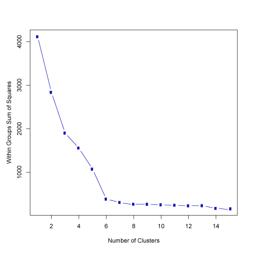
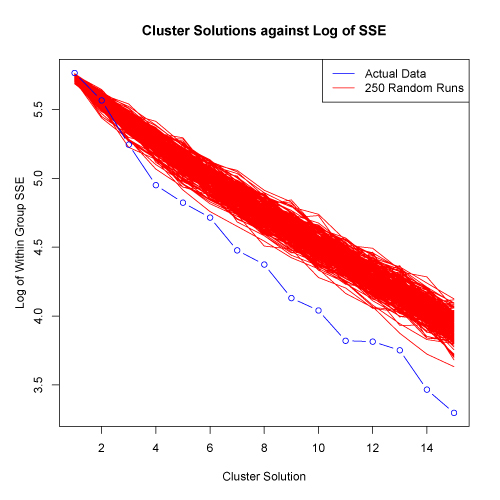
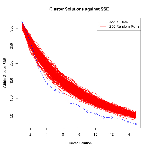
In many cases, however, there will not be such an obvious break in the distribution of SSE against cluster solutions. To help in such cases, the kmeans.R script conducts additional analyses to evaluate cluster solutions. Specifically, the script produces 250 randomized versions of the original input data, and calculates SSE against cluster solutions for the randomized data. The data is randomized by column, so each variable will have the same mean and standard deviation in both the actual and randomized matrices. If a data set has strong clusters, the SSE of the actual data should decrease more quickly than the random data as than cluster level goes up. Thus, the kmeans.R script plots SSE against the number of tested clusters for both the actual and 250 randomized matrices. Plots below are shown on both a log scale (left) and on a normal scale (right).


click to see images full size

In the examples shown above, the SSE for the actual data does decrease faster than the 250 randomized data sets. This suggests that the data set has structure and clusters are present. There is somewhat of a reduction in the rate of SSE decrease at about the 4 cluster solution. However, the "elbow" in the plot is not extreme and thus, further evaluation would be appropriate.

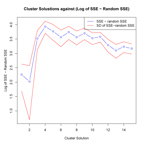
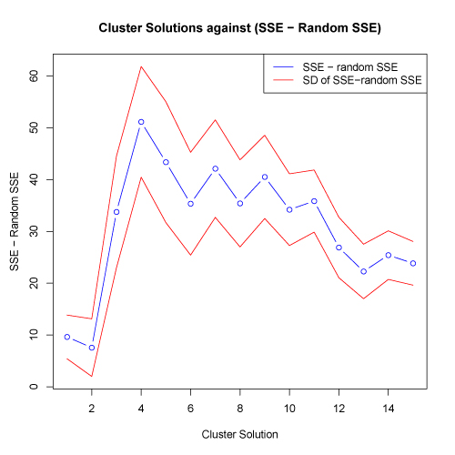
Another way to evaluate the appropriate cluster solution is to examine the absolute difference between the actual and random SSE against the tested cluster solutions. An appropriate cluster solution could be defined as the solution at which the actual SSE differs the most from the mean of the random SSE. To facilitate this comparison, the kmeans.R script displays the absolute difference between the actual and random (mean of all runs) SSE against the cluster solutions. One standard deviation above and below the mean absolute difference are also shown. Plots below are shown on both a log scale (left) and on a normal scale (right)


click to see images full size

In the plots above, the greatest absolute difference between actual and random SSE occurs at the 4 cluster solution. This suggests that this cluster solution may be an appropriate level to test. The fact that this cluster solution also coincides with the possible "elbow" in the plot of SSE against random SSE shown above provides additional information supporting this cluster solution.

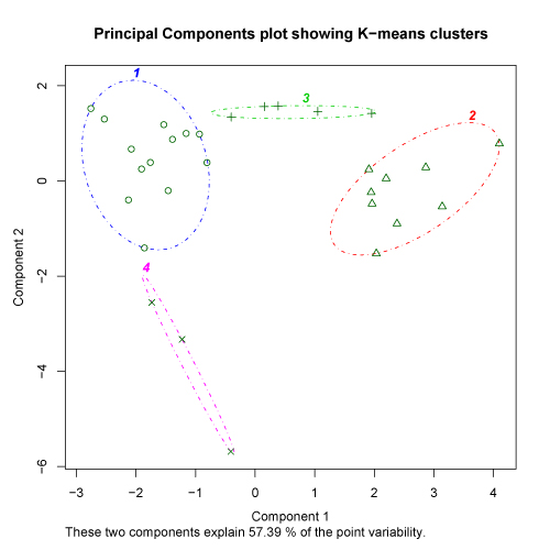
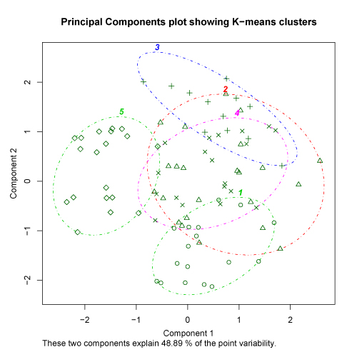
The kmeans.R script provides one final plot that may sometimes be useful in evaluating the proper cluster solution. After the user selects a cluster solution, the script conducts a principal components analysis on the original data set. Each sample is then displayed on a scatter plot of the first two principal axes of the PCA with the clusters outlined. If the clusters are strong at the selected level, there should not be substantial overlap in the distributions of the cluster outlines on the PCA plot. It is important to note that PCA plots may not be particularly useful for K-means analysis of data sets with a large number of samples or a large number of variables. There is no hard and fast rule for this, but the percent of the variability explained by the PCA provides some clue as to the potential utility of this approach. Check here for more details. The examples provided below show a PCA plot of relatively strong clusters (left) and somewhat weaker clusters (right).


click to see images full size

It is important to note that all of the procedures described above are simply heuristics to aid in choosing the appropriate clustering level. None of the specific recommendations shown here should be interpreted as strict rules. It is preferable that these suggestions are used as general guidelines. In your own analysis, you should evaluate the results of each of these procedures against each other and against your own knowledge of the data set that you are using. For additional information on K-means cluster analysis, and its applications in archaeology, see the references below.


Additional References

B. S. Everitt, S. Landau and M. Leese
2001 Cluster Analysis. London, Edward Arnold.

Kintigh, Keith W.
1990 Intrasite Spatial Analysis: A Commentary on Major Methods. In Mathematics and Information Science in Archaeology: A Flexible Framework, edited by A. Voorrips, pp. 165-200. Studies in Modern Archaeology. vol. 3. HOLOS-Verlag, Bonn.

Kintigh, K. W., and A. J. Ammerman
1982 Heuristic Approaches to Spatial Analysis in Archaeology. American Antiquity 47:31-63.

Script: